The INDEX function is a powerful tool in Excel that allows users to retrieve data from a specified range or array. This function can be used to quickly and easily find a specific value or cell within a large dataset. In this article, we will discuss how to use the INDEX function in Excel.

Syntax of the INDEX Function

Before we jump into the steps on how to use the INDEX function, let’s take a look at its syntax.
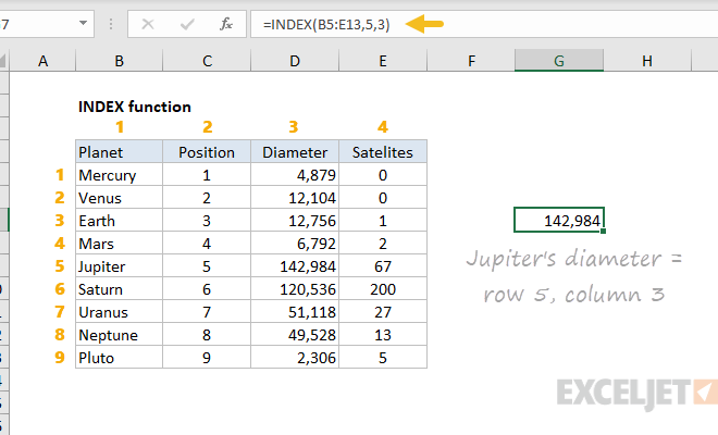
=INDEX(array, row_num, [column_num])

The “array” argument is the range of cells that we want to search for our data. This can be a single column or row, or an entire table.

The “row_num” arguments specify the row number within the array where we want to find the data. If we need to find data in a column, we can leave this argument blank or enter zero.

The “column_num” argument specifies the column number within the array where we want to find the data. If we need to find data in a row, we can leave this argument blank or enter zero.

Steps to Use the INDEX Function

Now that we understand the syntax of the INDEX function, let’s take a look at how to use it in Excel.

1. Start by typing “=INDEX(” in the cell where you want to display your result. This will start the formula.

2. Next, select the range of cells that you want to search for your data, and type a comma.

3. Enter the row number where you want to find your data, and type another comma.

4. Enter the column number where you want to find your data.

5. Finally, close the formula with a closing bracket, and press enter. The result will appear in the cell where you entered the formula.

For example, if you want to find the value of cell B3 in a table, the formula would be:
=INDEX(A1:D5, 3,2)

This formula will look for the value located in the third row and second column of the A1:D5 range.

Using the INDEX Function in Combination with Other Functions

The INDEX function can also be combined with other functions in Excel to create even more powerful formulas

For example, if you want to find the smallest value in a range of cells, you can use the INDEX function in combination with the MIN function.
=MIN(INDEX(A1:D5,0,3))

This formula will find the smallest value in the third column of the A1:D5 range.

Summary

The INDEX function is an essential tool in Excel that allows users to quickly and easily find specific data within a large dataset. This function can be used in combination with other Excel formulas to create even more powerful formulas. With the steps discussed above, you can start using the INDEX function in your Excel spreadsheets today.